Conditional Formatting is the method by which you can easily spot trends and patterns in your data using bars, colors, and icons to visually highlight important values. You can apply formatting to the content of cells depending on whether certain conditions are met.
From the Tabulate Spreadsheet:
- Select the cells that you want to apply conditional formatting to.
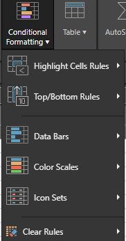
- From the Styles Ribbon, click Conditional Formatting. The following dropdown menu opens:
- This provides access to all the Conditional Formatting options. Select the desired options for your data.
- To highlight information based on specified criteria. For more information, see Highlight Content.
- To show highlight information based on top/bottom rules. For more information, see Highlighting based on Top/Bottom Rules.
You can apply conditional formatting:
You can also specify the appearance of:
You can also clear rules from either selected cells or the entire sheet. For more information, see Clear Rules.
Highlight Content
You can highlight content within cells that meets certain criteria. For example, if the content is greater or less than a defined value.
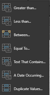
To access the Highlighting rules, select the Highlight Cells Rules menu option. The following dropdown menu is displayed:
Greater than
Selecting this option displays the following dialog:
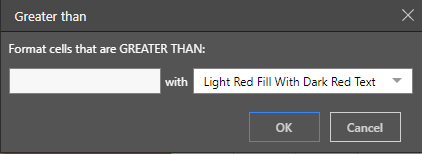
Enter the criterion to be tested in the left text box. In this case, we are testing whether the selected cell value is GREATER than the specified criterion. From the right dropdown menu, select the cell and text formatting to be used when the condition is met.
The criterion can be one of:
- A value (for example '100')
- A cell reference (for example 'B45')
- A formula using values and/or cell contents (for example 'F3*100'; 'F6/A1')
The selected cell will be formatted according to the selected style if the condition is met.
Less than
Selecting this option displays the following dialog:
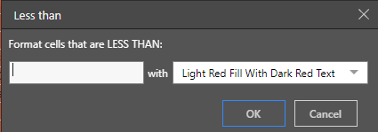
Enter the criterion to be tested in the left text box. In this case, we are testing whether the selected cell value is LESS than the specified criterion. From the right dropdown menu, select the cell and text formatting to be used when the condition is met.
The criterion can be one of:
- A value (for example '100')
- A cell reference (for example 'B45')
- A formula using values and/or cell contents (for example 'F3*100'; 'F6/A1')
The selected cell will be formatted according to the selected style if the condition is met.
Between
Selecting this option displays the following dialog:
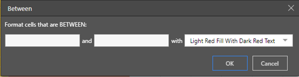
Enter the criteria to be tested in the text boxes. In this case, we are testing whether the selected cell value lies BETWEEN the specified criteria. From the right dropdown menu, select the cell and text formatting to be used when the condition is met.
The criterion can be one of:
- A value (for example '100')
- A cell reference (for example 'B45')
- A formula using values and/or cell contents (for example 'F3*100'; 'F6/A1')
The selected cell will be formatted according to the selected style if the condition is met.
Equal To
Selecting this option displays the following dialog:
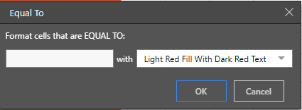
Enter the criterion to be tested in the left text box. In this case, we are testing whether the selected cell value is EQUAL to the specified criterion. From the right dropdown menu, select the cell and text formatting to be used when the condition is met.
The criterion can be one of:
- A value (for example '100')
- A cell reference (for example 'B45')
- A formula using values and/or cell contents (for example 'F3*100'; 'F6/A1')
The selected cell will be formatted according to the selected style if the condition is met.
Text that contains
Selecting this option displays the following dialog:
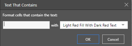
Enter the text value in the left text box. This value will be used to test if it is contained in the select text. In this case, we are testing whether the selected cell value CONTAINS any text specified. From the right dropdown menu, select the cell and text formatting to be used when the condition is met.
A Date Occurring
Note: This condition only applies to cells with a DATE value.
Selecting this option displays the following dialog:
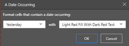
From the left dropdown menu, select the criterion to be tested. In this case, we are testing whether the selected cell value occurred:
- Yesterday
- Today
- Tomorrow
- Last 7 Days
- Last Week
- This Week
- Next Week
- Last Month
- This Month
From the right dropdown menu, select the cell and text formatting to be used when the condition is met.
Duplicate Values
Note: This tests for Unique or Duplicate values in the selected cells.
Selecting this option displays the following dialog:
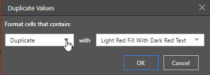
From the left dropdown menu, select the criterion to be tested, either:
- Duplicate
- Unique
From the right dropdown menu, select the cell and text formatting to be used when the condition is met.
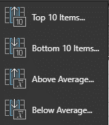
Highlighting based on Top/Bottom Rules
You can highlight cells whose values are:
- In the Top 10 of the selection
- In the Bottom 10 of the selection
- Are above the Average of the selected cells
- Are below the Average of the selected cells
Note: Select more than one cell for these functions to work correctly.
Selecting the Top/Bottom Rules option, displays the following menu:
Top 10 Items
Selecting the Top 10 Items, displays the following dialog:
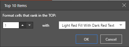
Use the up and down arrows to define the range required.
From the right dropdown menu, select the cell and text formatting to be used for cells whose content is in the RANGE specified.
Bottom 10 Items
Selecting the Bottom 10 Items, displays the following dialog:
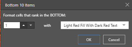
Use the up and down arrows to define the range required.
From the right dropdown menu, select the cell and text formatting to be used for cells whose content is in the RANGE specified.
Above Average
Selecting Above Average, displays the following dialog:
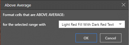
From the right dropdown menu, select the cell and text formatting to be used for cells whose contents are ABOVE AVERAGE for the selected cells.
Below Average
Selecting Below Average, displays the following dialog:
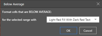
From the right dropdown menu, select the cell and text formatting to be used for cells whose contents are BELOW AVERAGE for the selected cells.
Data Bars
Selecting this option displays the following menu:
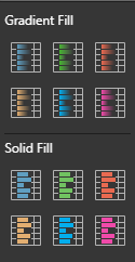
This enables you to select the gradient (or solid fill) options for data bars.
Color Scales
Selecting this option displays the following menu:
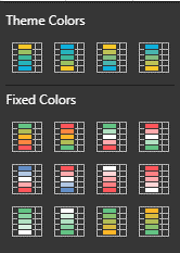
This enables you to select the color (either from the Theme or Fixed) options for data bars.
Icon Sets
Selecting this option displays the following menu:
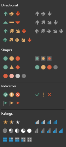
This allows you to select the Icon sets to be used in the Visualization.
Clear Rules
Selecting this option displays the following menu:
![]()
From this menu, you can clear the rules applied to selected cells or from the entire sheet.
Note: There is no 'undo' for this function.